Week 9

During this week, we derived the wave equation by taking the continuum limit of the discrete system (where there were a finite number of masses attached to a string). We started from the equation of motion for a single mass, which we derived last week:

$\ddot{y}_p = - \frac{T}{l m} \left[ 2y_p - y_{p-1} - y_{p+1} \right]$

which we can we write as

$\ddot{y}_p = - \frac{T l}{m} \frac{2 y_p - y_{p-1}-y_{p+1}}{l^2}$

then we use the fact that the second derivative of a function can be approximated by

$f''(x) \approx \frac{f(x+\epsilon) + f(x-\epsilon) - 2 f(x)}{\epsilon^2}$

this allows us to re-write the equation of motion as

$\frac{\partial^2 y}{\partial t^2} = \frac{T}{\mu} \frac{\partial^2 y}{\partial x^2}$

or, in terms of a velocity:

$\frac{\partial^2 y}{\partial x^2} = \frac{1}{v^2} \frac{\partial^2 y}{\partial t^2}$

So we now have the wave equation! This is our new favorite equation, and it is important to note that we obtained it from the behavior of a large number of coupled simple harmonic oscillators – that means that there is nothing intrinsically new here, but we have found a convenient formalism for dealing with systems with a large (essentially infinite) numbers of degrees of freedom.

Let us think about a “case study” of a string fixed at both ends (x = 0 and x = L).

We can now go about solving for the normal modes of oscillation. It is not difficult to check that the following is a solution:

$y_n (x,t) = A_n \cos (\omega_n t - \delta_n) \sin\left(\frac{2 \pi x}{\lambda_n}\right)$

Plugging this into the wave equation, we see that the wave equation is solved if $\frac{\omega_n}{v} = \frac{2 \pi}{\lambda_n}$

Further more, in order for $y_n$ to be zero at x=L, we need $\frac{2 \pi L}{\lambda_n} = n \pi$ , or $\lambda_n = \frac{2 L}{n}$ where n is any positive integer.

Thus, for a normal mode solution to the wave equation with the boundary conditions we have chosen (y(x=0) = y(x=L) = 0), we have:

$\lambda_n = \frac{2 L}{n} \text{ and } \omega_n = \frac{n \pi v}{L}$

Now since the wave equation is linear, any superposition of the normal mode solutions is also a solution, and we can write any motion of the string as

$y(x,t) = \sum_{n=1}^{\infty} A_n \cos\left[ \frac{n \pi v t}{L} - \delta_n \right] \sin \left[ \frac{n \pi x}{L} \right]$

(Of course always keep in mind that this only works sufficiently close to equilibrium, where the equation is linear – for large displacements/very jagged string configurations/etc, non-linear terms will be important, and will not be amenable to this type of analysis).

A good question that we will address next week is how to get out the unknown coefficients $A_n$ and $\delta_n$ . This process is referred to as Fourier analysis, in which the sum over normal modes is referred to as a Fourier Series expansion.

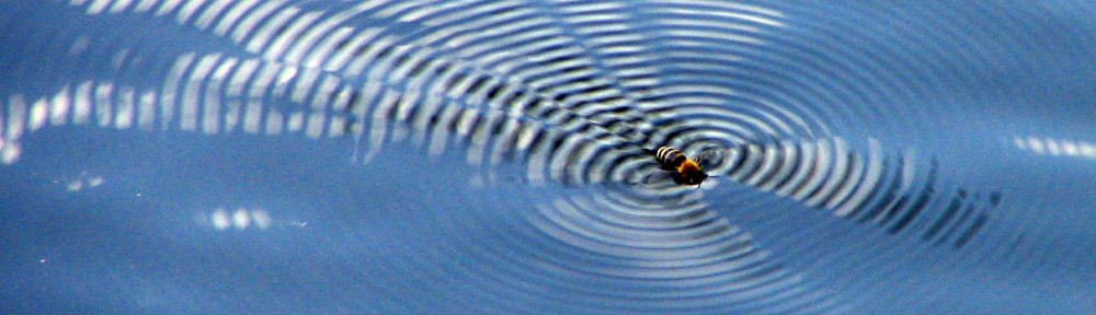
As a final note for this week, we note that we can derive the wave equation in a similar way for systems with spatial extent in more than one dimension. A string is 1 D, but we could consider a sheet/membrane, or the surface of water, as examples of media in which 2D waves can travel. Also, sound waves typically are transmitted in 3D spaces (like the classroom, or a shower that you might find yourself singing in).

In 2D, with transverse displacements from equilibrium characterized by a function $z(x,y,t)$ the wave equation is:

$\frac{\partial^2 z}{\partial x^2} + \frac{\partial^2 z}{\partial y^2} = \frac{1}{v^2} \frac{\partial^2 z}{\partial t^2}$

In 3D, where a sound wave is characterized by differences in the density of the ambient gas $\xi (x,y,z,t)$ , we have

$\frac{\partial^2 \xi}{\partial x^2} + \frac{\partial^2 \xi}{\partial y^2} + \frac{\partial^2 \xi}{\partial z^2} = \frac{1}{v^2} \frac{\partial y}{\partial t^2}$

In more than 1D, the patterns of nodes of the normal modes can become quite beautiful, and due to possible degeneracies (i.e. when a 2D medium is a square rather than a rectangle or some other shape), can have unexpected shapes. Our DEMO of the square plate with salt (or looked at with the strobe light) showed you some of this richness. Here is a picture of a guitar back when it is set into motion associated with one of its normal modes:

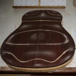
Normal modes are beautiful things, and in our engineering feats, it is of great value to understand the role that they play so that we can either eliminate them when they are problematic, or accentuate them when they are of value.

This weeks Mathematica notebook is here:

https://jhubisz.expressions.syr.edu/phy360/wp-content/uploads/sites/5/2016/11/Week-9.nb

In it, you should explore the transition from the discretuum to the continuum, and also seek to understand the structure of the normal modes (i.e. their shape, their relative frequencies, and the behavior of superpositions of normal modes).

Physics 360

Vibrations and Waves

Leave a Reply Cancel reply